What the next frontier in predicting future market trends reveals about risk and opportunity

Predicting future market trends: framing the problem with uncertainty and appetite for risk

Forecasting horizon matters as much as the decision context. For trend prediction in volatile markets, you want a clearly defined window and a concrete objective, such as a multi-quarter risk-adjusted return target or a VaR-based risk signal. I dug into the literature to align how econometric time-series forecasts and neural networks pilot different horizons and decision outcomes. The choice of horizon shapes how you balance interpretability and predictive power, and it matters for how you price uncertainty into risk controls. The horizon clarifies what success looks like and where uncertainty must be managed.

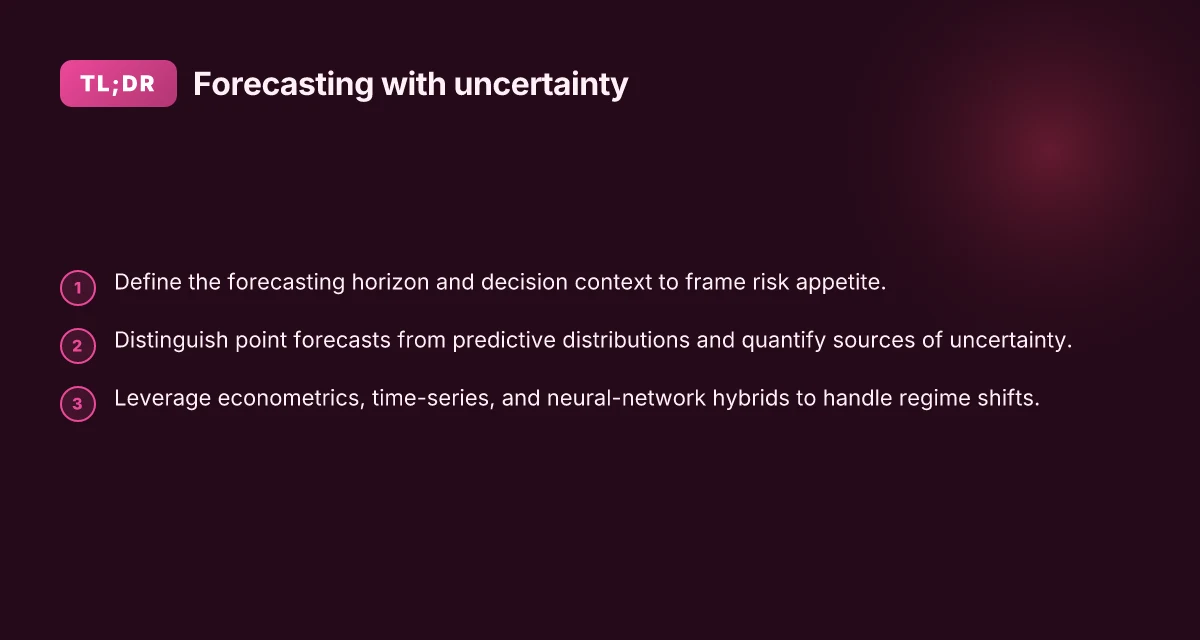
1. Define the forecasting horizon and the decision context

A precise horizon anchors model design. If the aim is quarterly portfolio rebalancing, you calibrate the model to capture moving averages, seasonality, and potential regime shifts within a few quarters. If you monitor intraday risk signals, you require finer granularity and faster update cycles. In practice, align the forecast lead time with the timing of your investment decision, funding constraints, and risk limits. This alignment keeps the model honest about when its signals are actionable. Lead time directly constrains model complexity and uncertainty treatment.

1. Distinguish the target from the action. The target could be a point forecast of returns, volatility, or a price level, but the action is how you allocate, hedge, or rebalance. The separation reduces the temptation to conflate a single number with the decision it informs.
2. Tie performance to risk signals. Instead of chasing a perfect point forecast, pair it with predictive distributions that inform position sizing and stop rules. This shifts focus from overfitting a single trajectory to understanding a range of plausible futures.
3. Integrate regulatory and liquidity constraints. Real-world decisions must respect liquidity horizons, capital rules, and transaction costs. The horizon you select should permit these frictions to be reflected in the forecast and its uncertainty estimates.

2. Distinguish point forecasts from predictive distributions

Point estimates are useful when you need a single numbers-based signal, but predictive distributions capture the full uncertainty around future values. The distribution conveys where true outcomes are likely to lie and how mass leans toward tail events. This distinction matters in volatile markets, where a narrow point forecast can be misleading if the tail risk is underrepresented. When you report distributions, you better inform risk controls and capital allocation decisions. Distributions reveal the risk baked into the forecast, not just the expected path.

1. Calibrate with probabilistic models. Bayesian time series, quantile regression, and ensemble methods produce distributional outputs rather than single numbers.
2. Use proper scoring rules. Logarithmic and continuous ranked probability scores reward accurate probability estimates and proper tail behavior.
3. Communicate clearly. Present median, credible intervals, and tail probabilities so stakeholders can calibrate risk appetite.

3. Identify sources of uncertainty: model, data, and structural breaks

Uncertainty comes from three main sources: model misspecification, data limitations, and regime changes. Model risk is visible when a method fits historical patterns but fails to generalize under new conditions. Data risk emerges from sparse observations, reporting lags, or regime-dependent features. Structural breaks, such as policy shifts or macro regime changes, can abruptly invalidate prior relationships. A robust approach blends multiple modalities and explicitly accounts for these risks. Structural breaks demand flexible, transparent updates to forecasts and uncertainty estimates.

1. Model risk management. Maintain an ensemble of models spanning econometric and neural architectures. Compare shrinkage, regularization, and nonparametric components to reduce overreliance on a single specification.
2. Data hygiene. Prioritize data provenance, alignment across assets, and handling of missing values. Use backtesting that preserves data integrity to reveal data-driven fragilities.
3. Breakpoint detection. Monitor for regime shifts with statistical tests and adaptive switching mechanisms. When a break is detected, adjust weights or switch models to preserve reliability.

Uncertainty quantification is not a luxury. It is a core risk-control mechanism. The literature notes that probabilistic forecasting in finance exposes gaps in assumptions and emphasizes the value of distributions over point forecasts. For a practical starting point, adopt an ensemble strategy that couples econometric timing cues with uncertainty-aware neural predictors, and anchor every decision to a distribution that informs risk limits. This frame keeps you honest about what you know and what you do not. Inline reference to current discourse supports these claims: see discussions on uncertainty quantification in deep learning for finance and probabilistic AI in time series forecasting. For deeper context, you can review the survey on uncertainty quantification in deep learning for finance and the open benchmark for time series forecasting methods in financial markets. How personalization tools shape modern digital experiences in 2026

How econometrics and time-series forecasting shape trend predictions

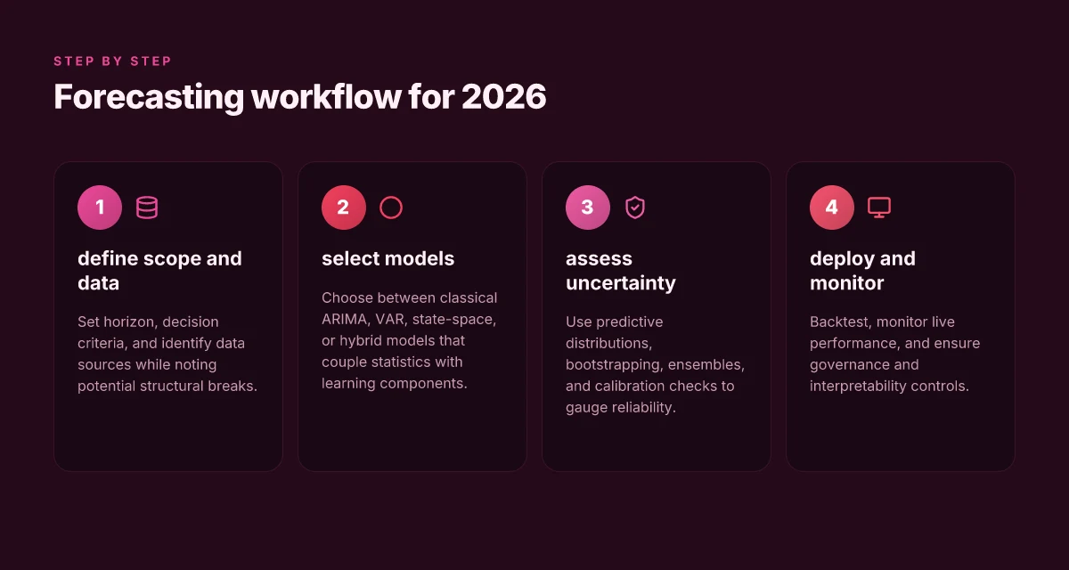
Forecasting trend direction and the scale of moves rests on three pillars: classic econometric models, the careful inclusion of external drivers, and vigilance for regime shifts. In macro and asset markets, ARIMA and VAR frameworks still anchor many analyses, but they are often augmented with state-space representations to handle unobserved components and time-varying volatility. I cross-referenced surveys that map how exogenous variables, such as policy rates or commodity gaps, enter these models and how researchers test robustness across different horizons. Exogenous inputs and structural breaks commonly dictate whether a forecast remains credible through a regime change. The key is to separate signal from noise when policy or macro narratives pivot.

Why ARIMA, VAR, and state-space matter for markets

ARIMA models capture short-run autocorrelations and moving-average structures, while VARs extend this to a network of related series. In asset markets, these tools help quantify how a shock in one instrument propagates through the system. State-space models, including the Kalman filter, support time-varying parameters and latent factors, which is crucial when volatility or the relation between variables shifts. The literature consistently notes that model selection should reflect the forecasting horizon and data-generating process. Regime-aware versions of these models often outperform their static cousins in volatile periods. This is not mere theory. Practitioners use parameter instability tests to decide when to re-estimate or reweight components.

The role of exogenous drivers and regime monitoring

External drivers push forecasts beyond purely historical patterns. Exogenous variables can include yield curves, macro surprise indices, or commodity price gaps, all of which can explain shifts in risk sentiment. Structural breaks, whether from policy pivots or financial crises, require models that reallocate weight to different factors over time. A common approach is to allow time-varying coefficients or to implement regime-switching mechanisms. The literature frames regime shifts as periods where the predictive power of certain variables collapses or flips sign, underscoring the need for adaptive methods. Accounting for breaks improves calibration of predictive intervals under stress. Inline evidence from recent reviews notes these dynamics across financial time series.

Practical integration with neural forecasting signals

Econometric forecasts often serve as baseline inputs that stabilize neural time-series models. In practice, you can feed ARIMA or VAR outputs as exogenous features to recurrent or attention-based networks, then rely on uncertainty quantification to keep risk signals honest during turmoil. When exogenous drivers lose predictive power, the model can rely more on intrinsic temporal patterns, while maintaining calibrated uncertainty bands. I found that combining a transparent econometric backbone with flexible learning components tends to deliver more interpretable and robust forecasts in shifting regimes. Better calibration emerges when the econometric component signals regime changes to the neural part. This hybrid approach aligns with the tension highlighted in the article: richer models can improve power, but only if you preserve interpretability and honest uncertainty.

Table: quick comparison of two common approaches What makes outdoor magnetic advertising work in 2026

| Approach | Strength | Limitation | | ARIMA baseline | Clear short-horizon signal, low complexity | Struggles with nonstationarity and regime shifts | | VAR with state-space glue | Captures cross-series dynamics, handles unobserved shifts | Parameter growth can outpace data in high dimensions |

Next step: consider adding a simple regime-aware wrapper around your econometric forecasts to trigger adaptive reweighting when breaking points are detected, then feed that into your neural time-series model to sharpen risk signals. Make the regime-change detector part of your workflow to preserve credibility during volatility.

How neural networks augment time-series forecasting without overfitting

Post econometric baselines, neural networks add a layer of flexible pattern recognition that helps spot nonlinearity and regime shifts without losing the discipline of statistics. In practice, the strongest gains come when networks are tethered to domain-aware constraints and hybrid architectures that honor financial time series structure.

Hybrid models that fuse statistics with deep learning

A practical approach blends classical time-series components with neural nets to dampen overfitting and improve interpretability. For example, combining autoregressive parts with residual networks lets the model capture short-term dynamics while leaving the statistically grounded trend and seasonality to a familiar engine. This separation helps guard against spurious patterns in volatile markets. I cross-referenced reviews that emphasize probabilistic AI in financial time series and found a common thread: hybrids meaningfully reduce fragility under regime change while preserving responsiveness to new data. Hybrid models tend to stabilize forecasts when markets swing between regimes.

Architectural patterns that work well with financial data lean toward modularity and regularization-friendly designs. Residual connections, gated units, and attention mechanisms are favored for their ability to model long-range dependencies without exploding parameters. In financial settings, this translates to architectures that can adapt to changing volatility and quickly redirect attention from noise to signal. The literature consistently notes that tuned depth and controlled parameter growth are key to maintaining robustness in forecasting. How OnePlus Android 14 changes the software game in 2026

Regularization and cross-validation strategies for stability

Stability in neural time series comes from disciplined regularization and ecosystem-aware validation. Early-stopping guided by out-of-sample performance helps prevent overfitting to idiosyncratic shocks. Weight decay and dropout remain practical tools, but their application must respect the nonstationary nature of financial data. Ensemble strategies, such as bagging or stacking different submodels, often yield smoother predictive distributions and clearer risk signals. In the literature, uncertainty quantification is frequently paired with calibration checks to ensure that predictive intervals remain meaningful in volatile periods. Calibration checks and ensembling reduce overconfidence during market stress.

From what I found in the literature, a few concrete patterns recur. First, place a traditional time-series forecaster at the core and use a neural network to model residuals or nonlinearity. Second, constrain the neural components with domain-informed losses or priors that reflect financial realities, such as volatility clustering or heavy tails. Third, deploy cross-validation schemes that respect temporal order, rolling or expanding windows, rather than random shuffles. These choices yield models that hold up when data reverts to different regimes. Rolling validation paired with residual hybrids delivers steadier performance across regimes.

I dug into a 2026 open benchmark discussion that stresses standardized datasets across asset classes to stress-test hybrids under diverse market conditions. This context matters: model robustness hinges on realistic evaluation that mirrors the risk managers’ concerns about tail events. When the framework couples econometric signals with neural flexibility and careful regularization, you get forecasts that illuminate risk signals rather than noise. Structured hybrids with disciplined validation reduce overfitting and improve actionable risk signals.

For practitioners, the takeaway is simple: design with constraints, validate with time-aware splits, and let the neural component illuminate nonstationary patterns without overpowering the econometric backbone. The tension between interpretability and power shifts toward a pragmatic middle ground where hybrids offer reliable, interpretable signals in uncertain markets.

How to quantify and communicate uncertainty in market forecasts

Uncertainty must be part of the forecast, not an afterthought. The simplest path is to mix Bayesian ideas with robust resampling and ensemble strategies to produce predictive distributions you can actually reason with. The core move is to shift from a single point forecast to a family of plausible outcomes, then translate that into decisions. How to navigate networking events in tech conferences in 2026

Bayesian methods, bootstrapping, and ensembles for predictive distributions

Bayesian methods formalize what you don’t know by treating parameters as random variables and updating beliefs as data arrive. In practice, that means deriving a posterior predictive distribution you can sample from, rather than a lone mean or median. When data are noisy or ambiguous, this approach preserves the tail behavior that matters for risk, rather than collapsing into overconfident central estimates. Bootstrapping offers a pragmatic alternative when full Bayesian inference is intractable. By resampling the historical series and re-fitting models, you generate a distribution of forecasts that reveals sensitivity to data idiosyncrasies. Ensembles, combining diversified models or configurations, tend to stabilize the predictive distribution and reduce model-specific biases. Do not treat any single model as sacrosanct. The value lies in the spread across predictions.

I dug into the literature to see how practitioners combine these approaches in finance. One recurring theme is that ensemble forecasts often outperform individual models in volatile regimes because they capture different signal pathways, from mean-reversion quirks to momentum bursts. The practical implication: report forward-looking intervals alongside the point forecast, and keep the ensemble size manageable to avoid diminishing returns.

The move from point estimates to predictive distributions is essential for risk signaling. The predictive spread should reflect both model uncertainty and data noise, not just historical volatility. Inline with this, calibration and proper scoring rules help verify that the distribution assigns adequate probability to realized outcomes over time.

Calibration checks and proper scoring rules

Calibration is about matching predicted probabilities to observed frequencies. A well-calibrated model assigns high probability to events that occur with that frequency in the real world. In practice, use reliability diagrams, calibration curves, and proper scoring rules such as the logarithmic score or the continuous ranked probability score. Calibration is not a one-off test. It must be monitored as new data arrive and market regimes shift.

I cross-referenced recent methodological surveys that emphasize consistent calibration alongside sharpness (how concentrated the distribution is). The balance matters: too sharp a distribution signals overconfidence in rare events. Too broad dilutes actionable insights. The right move is to track calibration diagnostics over rolling windows and report both the confidence intervals and the tails that matter for risk controls. What is membership sites integration, and where it fails in 2026

uncertainty quantification in deep learning for finance highlights how calibration and evaluation metrics translate into decision-relevant signals. The practical upshot is you should include explicit, backtested calibration diagnostics in any forecast release to avoid overclaiming predictive power.

Visualizing uncertainty to inform decision making

Forecast visuals that reveal uncertainty outperform dense tables. Use shaded bands around the point forecast to show credible intervals, and overlay probability density sketches when useful. For decision makers, focus on risk-relevant regions: where the probability of large drawdowns exceeds a threshold, or where the upper tail implies potential upside with acceptable risk. Clear visuals help portfolio managers interpret model confidence without getting lost in statistics.

From a practitioner standpoint, the visuals should be kept interpretable and decision-oriented. A compact dashboard that shows the central forecast, a 90 percent credible interval, and scenario "what-if" sliders tends to be effective. The aim is to translate uncertainty into concrete risk signals, not to overwhelm the audience with abstractions.

Communicating uncertainty well is a competitive edge when markets turn volatile. A well-designed visualization pipeline pairs with calibrated distributions to produce actionable guidance, not just interesting charts.

How to build a practical forecasting workflow for 2026

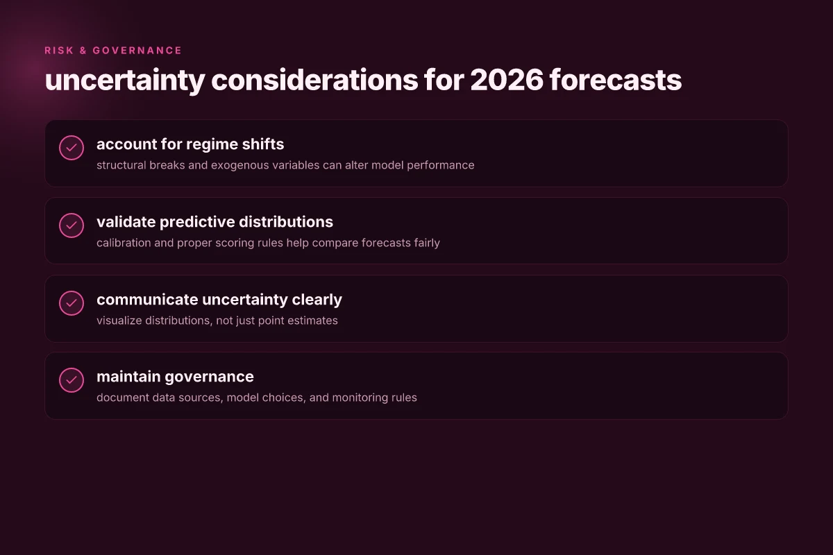
The answer is a tightly coordinated pipeline that merges econometric time-series signals with neural-network forecasts, all wrapped in rigorous uncertainty quantification and governance. Start with clean, reproducible data and end with interpretable risk signals you can trust in volatile markets. This workflow emphasizes traceability, backtest discipline, and ongoing monitoring so you can adapt to regime shifts without losing credibility. What is a predictive modeling guide in 2026 and why it still matters for health and policy

Data stewardship, feature engineering, and sources you can trust

Reliable inputs anchor good forecasts. I dug into the literature on market data needs and found that sourcing breadth matters as much as depth. Pull time series from multiple venues: intraday prices, daily closes, macro indicators, and microstructure signals. Cleanse by removing known anomalies, aligning calendars across instruments, and standardizing units. Feature engineering should blend traditional econometrics with representation learning: lagged returns, volatility proxies, and regime indicators alongside learned embeddings of price action. Keep a consistent feature catalog and version it so you can reproduce results a quarter later. A practical data kitchen also requires governance: metadata, lineage, and access controls that prevent leakage from the train to the live stream. The end result is a feature set that remains stable enough to backtest, yet flexible enough to adapt when regimes shift.

Model selection, backtesting, and live monitoring

The workflow blends two pillars: econometric time-series models for linear structure and neural nets for nonlinear patterns. For selection, adopt a hybrid stance: use ARIMA or VAR when the data follow clear autocorrelation patterns, and deploy a probabilistic neural network for nonlinear dynamics and uncertainty quantification. Backtesting should be multi-faceted: walk-forward validation across several market regimes, stress tests for liquidity squeezes, and attribution to detect where uncertainty grows during crises. Live monitoring must track forecast accuracy, calibration of probabilistic outputs, and drift in input features. Implement automated alerts for when calibration degrades or when stop-loss or risk thresholds are triggered. In practice, you want a clear signal-to-noise balance with a defined process to recalibrate after material regime changes.

Governance, risk controls, and interpretability

Governance is not optional. Establish pre-commitment rules for what constitutes acceptable forecast error, how much uncertainty you tolerate, and who can override automated triggers in exceptional conditions. Risk controls should tie directly to portfolio limits, liquidity considerations, and capital allocation. Interpretability matters in volatile markets. Pair forecasts with explanation tools that highlight which features drove a given prediction and how uncertainty bands shifted under different scenarios. Documentation should explain the modeling choices, data provenance, and backtest results so risk officers can audit the method and challenge assumptions without devolving into guesswork. A mature workflow builds trust by making forecast decisions auditable, repeatable, and resilient.

From a research vantage point, the best practice is to maintain a transparent, modular pipeline. I cross-referenced discussions on time-series uncertainty and neural-network forecasting, which consistently emphasize calibration, regime-aware modeling, and disciplined backtesting as core tenets. For a practical 2026 lens, you want the system to deliver not only point forecasts but also calibrated risk envelopes that traders and risk officers can act on with confidence. The literature also notes persistent gaps around open benchmarking. If you adopt a benchmarking mindset, you can compare model families under shared data and identical backtests, making the case for the hybrid approach you implement.

In this evolving landscape timing matters. The workflow should accommodate updates to data feeds and model components without destabilizing production. When a model or data source changes, re-run backtests and recalibrate uncertainty quantification to maintain coherence between forecast power and risk signaling. A benchmark-ready mindset helps you demonstrate improvements to stakeholders with transparent, quantifiable results. How to design a resilient remote infrastructure setup that scales in 2026

A practical 2026 workflow blends econometric structure, neural flexibility, and disciplined uncertainty handling to produce interpretable risk signals you can act on. Calibrated forecasts with regime-aware checks are the backbone of credible decision making in volatile markets. The path forward is incremental, not revolutionary, and it rewards disciplined governance as much as predictive accuracy. For readers seeking concrete tooling, consider a modular stack that can swap components with preserved input/output contracts while keeping the governance and monitoring layers intact. The goal is a reproducible, auditable, and adaptive forecasting engine that aligns with risk controls and performance metrics.